NumPy for DataScience

NumPy is a package for scientific computing in Python it provides a multidimensional array object for fast operations on arrays such as mathematical, logical, shape manipulation, sorting,selecting, I/O, discrete Fourier transforms, basic linear algebra, basic statistical operations and much more.

We have multidimensional lists in Python then Why NumPy?

Why NumPy over Python lists?

1. NumPy array are more compact than Python lists.

2. More efficient and fast in mathematical calculation for large data.

3. Vectorization

4. Broadcasting

Vectorization and Broadcasting

Vectorization is a technique of writing code without any explicit for-loops and indexing. When we want to multiply two arrays element wise we generally do :

>>> a = [[1,2,3],[4,5,6],[1,2,3]]
>>> b = [[3,2,1],[2,3,1],[1,2,3]]
>>> for i in range(3):
...  for j in range(3):
...   a[i][j] = a[i][j] * b[i][j]
... 
>>> a
[[3, 4, 3], [8, 15, 6], [1, 4, 9]]

To avoid any of these for-loops and indexing NumPy provides vectorization. So, what if they were NumPy array and not multidimensional lists.

>>> a = np.array([[1,2,3],[4,5,6],[1,2,3]])
>>> b = np.array([[3,2,1],[2,3,1],[1,2,3]])
>>> a * b
array([[ 3,  4,  3],
       [ 8, 15,  6],
       [ 1,  4,  9]])

Easy?

Broadcasting refers to implicit element wise operations(In simple terms). NumPy operations generally are performed element wise. To perform element wise operations array must be broadcasted or should be made of equal shapes. This conversion is done behind the scenes when you operate two array of unequal shapes. For eg :

>>> a = np.array([1,2,3])
>>> b = np.array([[3,2,1],[3,2,1]])
>>> a * b
array([[3, 4, 3],
       [3, 4, 3]])

For the above operation firstly ‘a’ i.e [1,2,3] was converted to [[1,2,3],[1,2,3]] then element wise operation took place between ‘a’ & ‘b’ . So, this example shows both Vectorization and Broadcasting.

Getting started

NumPy does not come with Python itself for installation you may refer the link. If you have successfully installed numpy then continue reading below.
Whenever you start your python script first you have to import numpy package to your code and then start working with numpy. To import numpy to your python script type the following:

import numpy as np

Here you import numpy module renamed as np .

This is enough for a brief description of numpy. Now, let’s get NumPy in action.

Basics of NumPy

NumPy arrays are ndarray objects which stands for n-dimensional arrays of homogeneous data types.

Creation

How to make a NumPy array?

1. A NumPy array can be made with a list by calling np.array(list,dtype) and passing a list to it specifying the data types. for further description on data types follow the link.

   >>> a = [[1,2,3],[4,5,6]]
   >>> arr = np.array(a,dtype=np.int32)
   >>> arr
   array([[1, 2, 3],
      [4, 5, 6]], dtype=int32)

2. A NumPy array with zeros all over can be made by calling np.zeros((rows,cols)) and specifying number of rows and columns.

   >>> np.zeros((3,2))
   array([[ 0.,  0.],
      [ 0.,  0.],
      [ 0.,  0.]])

3. A NumPy array with a particular value all over can be made by calling np.full((rows,cols),value,dtype) and specifying number of rows,columns,value to be filled with and data type.

   >>> np.full((3,2),5,dtype=np.int64)
   array([[5, 5],
      [5, 5],
      [5, 5]])

4. Similarly for making NumPy arrays with ‘1’ as a value call np.ones((rows,cols),dtype) specifying number of rows and columns with data type.

   >>> np.ones((3,2),dtype=np.int64)
   array([[1, 1],
      [1, 1],
      [1, 1]])

5. NumPy also provides a way to produce indentity matrix. To make a identity matrix call np.eye(dim) and specify the dimension.

   >>> np.eye(3)
   array([[ 1.,  0.,  0.],
      [ 0.,  1.,  0.],
      [ 0.,  0.,  1.]])

6. To make arrays with random numbers call np.random.random((rows,cols)) and specify number of rows and columns. This will create a numpy array with random numbers between ‘0’ and ‘1’.

   >>> np.random.random((2,3))
   array([[ 0.54718331,  0.89454271,  0.88606565],
      [ 0.27136812,  0.23676152,  0.49494242]])

Slicing

Slicing refers to selecting a particular part of an array by providing index ranges.

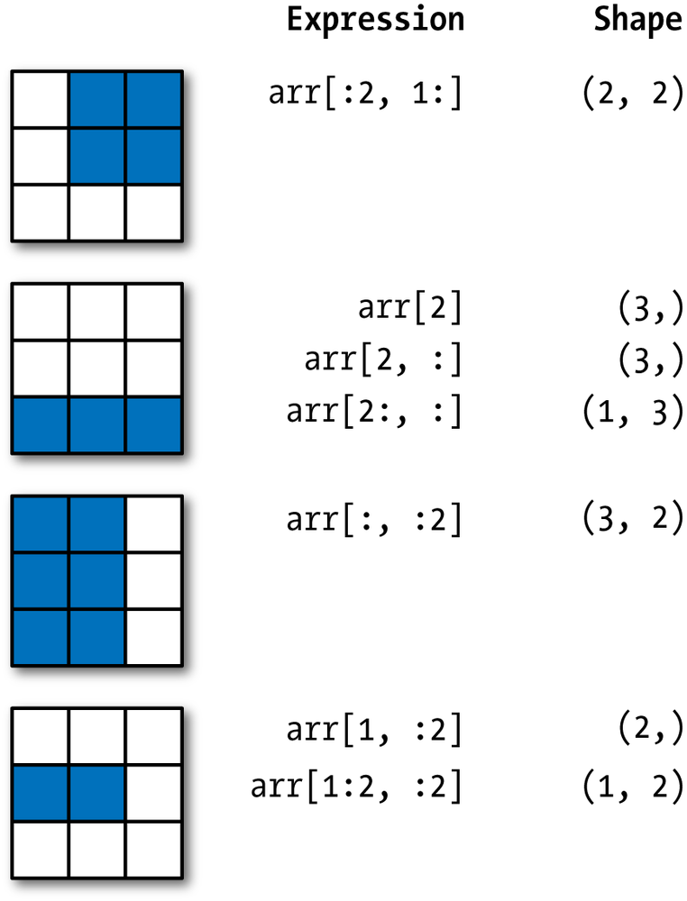
Specifying slices can extract a particular part of an array. We can specify a slice as array[begin_row:end_row,begin_col:end_col].

>>> arr
array([[ 1,  2,  3,  4],
       [ 4,  5,  6,  7],
       [ 8,  9, 10, 11],
       [12, 13, 14, 15]])
>>> arr[1:4,2:4]
array([[ 6,  7],
       [10, 11],
       [14, 15]])

Indexing starts at ‘0’ and end_row and end_col in not included. So here arr[1:4,2:4] means row(1) to row(3) and col(2) to col(3).

When we leave a index blank like arr[:3,1:] this automatically fills as starting or ending of row or column respectively.

>>> arr[:3,1:]
array([[ 2,  3,  4],
       [ 5,  6,  7],
       [ 9, 10, 11]])

A different way of slicing is arr[start:stop:step]. If you write arr[1:10:2] this means starting from index 1 to index 9 taking 2 as a step so to display indexes 1,3,5,7,9.

>>> arr
array([ 0,  1,  2,  3,  4,  5,  6,  7,  8,  9, 10])
>>> arr[1:10:2]
array([1, 3, 5, 7, 9])

We can also extract elements with specifying logical operations. arr[arr>4] this will give all elements greater than 4 in arr.

>>> arr
array([ 0,  1,  2,  3,  4,  5,  6,  7,  8,  9, 10])
>>> arr[arr>4]
array([ 5,  6,  7,  8,  9, 10])

Operations

NumPy provides various mathematical, logical, statistical operations with efficiency and speed. Some are listed below :

>>> array_1
array([[1, 2, 3],
       [4, 5, 6],
       [7, 8, 9]])
>>> array_2
array([[7, 8, 9],
       [4, 5, 6],
       [1, 2, 3]])

1. Adding two arrays with np.add().

>>> np.add(array_1,array_2)
array([[ 8, 10, 12],
       [ 8, 10, 12],
       [ 8, 10, 12]])

2. Subtracting two arrays with np.subtract().

>>> np.subtract(array_1,array_2)
array([[-6, -6, -6],
       [ 0,  0,  0],
       [ 6,  6,  6]])

3. Multiplication element wise with np.multiply().

>>> np.multiply(array_1,array_2)
array([[ 7, 16, 27],
       [16, 25, 36],
       [ 7, 16, 27]])

4. Dividing element wise with np.divide().

>>> np.divide(array_1,array_2)
array([[ 0.14285714,  0.25      ,  0.33333333],
       [ 1.        ,  1.        ,  1.        ],
       [ 7.        ,  4.        ,  3.        ]])

5. Matrix multiplication with np.dot().

>>> np.dot(array_1,array_2)
array([[ 18,  24,  30],
       [ 54,  69,  84],
       [ 90, 114, 138]])

6. Square root element wise with np.sqrt().

>>> np.sqrt(array_1)
array([[ 1.        ,  1.41421356,  1.73205081],
       [ 2.        ,  2.23606798,  2.44948974],
       [ 2.64575131,  2.82842712,  3.        ]])

7. Exponential constant to the power of element in array with np.exp().

>>> np.exp(array_1)
array([[  2.71828183e+00,   7.38905610e+00,   2.00855369e+01],
       [  5.45981500e+01,   1.48413159e+02,   4.03428793e+02],
       [  1.09663316e+03,   2.98095799e+03,   8.10308393e+03]])

Statistical operations

Statistical Operations are very much optimised when we use NumPy array.

>>> array_1
array([[1, 2, 3],
       [4, 5, 6],
       [7, 8, 9]])
>>> array_2
array([[7, 8, 9],
       [4, 5, 6],
       [1, 2, 3]])

Note:- Axis value is for computing operation along rows when axis=1 and along columns when axis=0

1. Computing mean with np.mean(array,axis) specifying name of array and axis.

>>> np.mean(array_1,axis=1)
array([ 2.,  5.,  8.])

2. Computing median with np.median(array,axis) specifying name of array and axis.

>>> np.median(array_1,axis=0)
array([ 4.,  5.,  6.])

3. Computing sum with np.sum(array) for sum of entire array and np.sum(array,axis) for a particular axis.

>>> np.sum(array_1)
45
>>> np.sum(array_1,axis=1)
array([ 6, 15, 24])

4. Sorting a array with np.sort(array,axis).

>>> np.sort(array_1,axis=1)
array([[1, 2, 3],
       [4, 5, 6],
       [7, 8, 9]])

5. Unique values across array with np.unique(array).

>>> np.unique(array_1)
array([1, 2, 3, 4, 5, 6, 7, 8, 9])

Some Other Operations

After a quick basic, these are some more NumPy operations that are required for getting into DataScience.

>>> array_1
array([1, 2, 3, 4, 5])
>>> array_2
array([4, 5, 6, 7, 8])

1. To find intersection of two 1-dimensional arrays with np.intersect1d(array_1,array_2).

   >>> np.intersect1d(array_1,array_2)
   array([4, 5])

   
   

2. To find Union of two 1-dimensional arrays with np.union1d(array_1,array_2).

   >>> np.union1d(array_1,array_2)
   array([1, 2, 3, 4, 5, 6, 7, 8])

   
   

3. To find elements in array_1 not in array_2 with np.setdiff1d(array_1,array_2).

   >>> np.setdiff1d(array_1,array_2)
   array([1, 2, 3])

   
   

4. Boolean (True or False) for elements in a array contained in other with np.in1d(array_1,array_2).

   array([False, False, False,  True,  True], dtype=bool)

   
   

5. Find Maximum element in a array with np.max(array,axis).

   >>> array_1 = np.array([[1,2,3],[4,5,6],[7,8,9]])
   >>> np.max(array_1,axis=1)
   array([3, 6, 9])

   
   

6. Find minimum element in a array with np.min(array,axis).

   >>> np.min(array_1,axis=1)
   array([1, 4, 7])

   
   

7. Generate sequence of numbers from 0-value with np.arange(value).

   >>> np.arange(10)
   array([0, 1, 2, 3, 4, 5, 6, 7, 8, 9])

   
   

8. Reshape a array with array_name.reshape(rows,cols) specifying number of rows and columns .

   >>> array_1
   array([[1, 2, 3],
      [4, 5, 6],
      [7, 8, 9]])
   >>> array_1.reshape(9,1)
   array([[1],
      [2],
      [3],
      [4],
      [5],
      [6],
      [7],
      [8],
      [9]])

   Note:- number of elements in the array must be eqaul to rows * cols
   

9. To apply logical operation on an array and fill values according to bool returned with np.where(logic,True_fill,False_fill) here logic specifies the logical operation wheread True_fill and False_fill are values to be filled when True or False is returned respectively.

   >>> array_1
   array([[1, 2, 3],
      [4, 5, 6],
      [7, 8, 9]])
   >>> np.where(array_1>4,1,0)
   array([[0, 0, 0],
      [0, 1, 1],
      [1, 1, 1]])

   
   

10. To Generate random integers between a range with np.random.randint(low,high,size) here low and high are the ranges and size is the number of elements needed.

    >>> np.random.randint(0,50,15)
    array([38, 14, 28,  1,  5,  4, 21, 24, 33,  7, 26, 47, 49,  9, 13])

    
    

11. Generate random permutation of an array with np.random.permutation(array) .

    >>> np.random.permutation(array_1)
    array([[1, 2, 3],
       [4, 5, 6],
       [7, 8, 9]])

    
    

12. To return equispaced elements between a range np.linspace(start,end,elements) here start and end is the range and elements is the number of elements required.

    >>> np.linspace(10,30,10)
    array([ 10.        ,  12.22222222,  14.44444444,  16.66666667,
        18.88888889,  21.11111111,  23.33333333,  25.55555556,
        27.77777778,  30.        ])

13. Concatenation of two arrays with np.concatenate([array_1,array_2],axis).

    >>> array_2 = np.random.rand(2,2)
    >>> array_1 = np.random.rand(2,2)
    >>> np.concatenate([array_1,array_2],axis=1)
    array([[ 0.49812363,  0.06835159,  0.37823207,  0.97684743],
       [ 0.615256  ,  0.06289467,  0.10976521,  0.09625162]])

Shape

One of the important data member of ndarray is shape, We often need to know the shape of our numpy array. For this we use array_name.shape.
For 1D array, return a shape tuple with only 1 element (i.e. (n,)).
For 2D array, return a shape tuple with only 2 elements (i.e. (n,m)).
For 3D array, return a shape tuple with only 3 elements (i.e. (n,m,k)).

>>> array_1
array([0, 1, 2, 3, 4])
>>> array_1.shape
(5,)
>>> array_2
array([[ 1.,  1.,  1.],
       [ 1.,  1.,  1.]])
>>> array_2.shape
(2, 3)
>>> array_3
array([[[ 0.,  0.,  0.],
        [ 0.,  0.,  0.]]])
>>> array_3.shape
(1, 2, 3)

Okay, that was the last one. Hope you understood everything but if not you can anytime search the numpy documentation here.

Conclusion

A warm up with numpy is done to get started with data science.